The character of a sound is controlled by the three distinct properties pitch, loudness and timbre. These are named the three basic parameters of a sound. All three are dynamic in nature, changing and developing gradually over the time the sound is heard. So, a distinct sound is characterized by how pitch, loudness and timbre each develop over time. The musician or composer controls how these developments will be by either dynamically and expressively playing the parameters or describing their temporal developments in a score on paper, a computer file or even a computer program.
Whenever a sound is heard there will always be sensations of pitch, loudness and timbre. Additionally a sound has a certain starting point and a certain end point in time, formally the time between two adjacent periods of zero loudness, giving a certain duration to the sound. Some composers name sound duration a fourth parameter of sound. But as the sound duration is already implicit in the description of how the loudness of the sound develops over time, this parameter can be discarded when the developments of the three basic parameters are described well enough. Of course this is of much more concern to composers, who have to somehow describe sounds in a score, than to a musician who simply wants to play the sound.
A musical sound (which is just any sound that is used in a piece of music) doesn’t necessarily need to have the distinct single pitch of a single piano or organ note. There can be more pitched components in a sound, like in a chord. Additionally, these pitched components don’t necessarily have to have a harmonic relationship, just think of the ‘enharmonic’ sounds of certain drums and percussive instruments. In this class of sounds there still can be one pitched component that is perceived as the dominant pitch, enabling the sound to be tuned to other sounds. An example of such a sound is the sound of a timpani drum.
Another class of sounds is named the pitchless sounds, like the sound of falling rain or ocean waves. In fact pitchless sounds are an assembly of many pitched components, but there are so many components that the human ear cannot perceive their distinct pitches any more. The components melt into one single ‘pitchless’ sensation. And although there is no sense of a definite pitch in pitchless sounds, there can be a strong sense of very characteristic timbres. Noise is the textbook example of a pitchless sound. In nature noise is created by processes that are in essence chaotic, meaning that there is a definite order in the process, but the order is too complex for the human mind, it cannot detect the order and will even have a hard time to concentrate on one of the individual components. Think of a waterfall and how the turbulence of the falling water creates the sound. It is impossible to follow all the terbulent water movements by eye or ear, but there is a definite physical reason why the water at a certain moment falls and sounds like it does.
In noise there are so much pitched components present that each of them literally drowns in the overall sound. Still, this noise might be produced by a well defined and in essence simple and orderly executed process. Noise might appear random, but that doesn’t mean it is really random, in fact there might be all sorts of statistical properties in the noise. Later on it will be shown how these statistical properties can affect the many possible timbres of noise based sounds.
An interesting moment is when something that is perceived as an orderly process develops towards the state where it is perceived as chaotic. In the moment of the transition from order to chaos the human mind can still concentrate on a single component of the sound, but the mind will start trying to skip from component to component. An interesting example can be heard once a year when visiting the Frankfurter Musikmesse, where one exposition hall is exclusively dedicated to the grand piano. There might be a hundred or so piano’s on display, ready to be played by potential buyers. On the busiest moments at the fair all piano’s are being played. Of course this creates a huge and totally chaotic sound, aptly named a cacophony. By taking a strategic position somewhere in the hall and listening to the overall sound there is these short moments one suddenly recognizes a bit of Beethoven in the cacophony, immediately dissolving into some ragtime and then dissolving into cacophony again. It is virtually impossible to catch and hold on to the moment when something is recognized in the cacophony.
When a sound is heard it will always give a distinct sensation of timbre. Timbre plays an important role in recognizing the sound. The synthesizer is specifically designed to be able to generate a vast range of timbres. Timbre as a phenomenon is created by a collection of partials, similar to how molecules are created by a collection of atoms. In the nineteenth century the physicist Helmholz has proved that a singular pitched sound has a series of possible partials. If these partials are harmonically related they are named harmonics or overtones. All natural sounds have some or more partials. Only by electronic means can a sound be created that consists of only one single partial, the one that is named the fundamental. The waveform that creates this sound is named a sinewave. As this sound has no extra partials to give it a timbre, it can be said that the sound of a sinewave has no timbre, similar to saying that distilled water has no taste.
Working on the timbre of a sound is the most laborious part of sound design. Human hearing is incredibly sensitive to the most subtle changes in timbre. Additionally there is the tendency to adhere some association or sense of meaning to the intonation of sounds. The same sentence of spoken words can change from a question to a command by only changing the intonation, e.g. by slightly changing the pitch development in the words. In certain circumstances timbral effects are used to work on the human emotion. Examples are religious music, shamanistic incantations, and the like. Psycho-acoustics might also play an important role, especially when a sense of spaciousness is required. Another important aspect of timbre is legibility, or how easy it is to isolate the sound in between other sounds, in order for the mind to recognize it and give it some meaning. Some aspects in timbre have the ability to mask away aspects in other sounds, reducing their legibility. This is of great importance during the mastering process of a music recording when the mastertape is made which will be used as the source for submitting the music to vinyl or a CD. In the mastermix it might turn out that instruments conflict with each other, reducing each others legibility or presence. The regular approach is to use compressors and equalization functions on the mixing desk to improve the mix. However, it is common sense to think things out before initial recordings are being made, so these conflicts in legibility occur to a much lesser extend. A good orchestration or arrangement for a piece of music can emphasize the melodic or timbral structures by a well balanced choice of sounds that do not mask each other away, but instead tend to emphasize each other musically.
Loudness is how an individual perceives the volume of a sound at a certain sound pressure level or SPL. This perception can differ from person to person, as not everybody has the same sensitivity for different registers in the audio range. Also, a sound might be so low in volume that the ear doesn’t perceive it any more, while a measurement device would still prove it present. The point where the volume is so low that the ear ceases to hear the sound is named the threshold of audibility. This threshold differs for person to person and for different pitches. In general the threshold for the higher pitches is raised when a person is getting older, until finally deafness for this pitch range occurs. Note that when the threshold is raised it means that a louder volume is needed for the sound to be heard. Like the threshold of audibility is the lower limit of the hearing range, there is also sort of an upper limit to this range. When the sound pressure exceeds this limit a severe pain in the ears is felt. Increments in volume are no longer heard above this level, as it is overruled by the pain sensation getting worse. Excessive sound levels can permanently damage one’s ears, resulting in deafness. Very loud volume levels that do not yet induce pain in the ears will also cause deafness over time. So, great care must be taken with loud volume levels, damage to the ears caused by loud levels is permanent and a great disaster for a musician, compare it to when a painter gets blind. It is very wise to protect one’s ears during performing live to avoid possible future hearing damage. Headphones can also produce a lot of sound pressure on the ear, which may result in ear damage as well. Never take any risk with loud volumes. It is better to keep a comfortable volume level, not too soft but also not too loud. At a comfortable volume level one can also hear the most detail in sounds. In general a good volume level for the studio is when the sound can be easily heard and only a slight concentration is needed to hear a specific detail in the sound. When the volume level is either too low or too loud more concentration is needed. Find a balanced loudness level that feels comfortable and doesn’t tire after some hours.
Handling volume levels requires experience, as several psycho acoustic principles are involved and it takes getting used to hearing these principles at work. When designing sounds that need to be played expressively it is important to keep these principles in mind. Psycho acoustics is a science by itself and it goes beyond this book to delve into the details. Still, some basic examples will be given in the following paragraph, as these examples are many times the key to a good sound.
The human mind has the capacity to mute sounds from the surroundings. These ambient sounds are registered by the ear, but they don’t enter into the awareness. This has to do with how the mind concentrates on what it is doing. Sudden changes in volume in these sounds will attract the attention. Another effect is that when the volume reaches a certain loudness level people are forced to listen to it. But this doesn’t mean that they listen attentively. Softer loudness levels are better in keeping the focused on the sound, as a little more effort is required to listen to the sound. It is advisable to keep the volume at a reasonable level in a small or medium sized listening room or when performing at a small club.
There has been research on how loud certain frequencies have to be in order to be perceived at a uniform loudness level by the mind. So, how the SPL for a given frequency range has to change to be perceived equally loud as another frequency range.This can be plotted in a curve that is named an equal loudness curve. This curve is different from person to person, but when a lot of individual curves are averaged a curve results that is named the Fletcher-Munson curve. This curve reveals that in general the human ear is the most sensitive to volume changes in the 2kHz to 5kHz region, while being only moderately sensitive to volume changes in the bass region. This curve can have an impact on a mix, as when the mix is made at a relatively low loudness level, the 2kHz to 5kHz region might sound too loud when the recorded mix is played back at a much higher loudness level, making the overall sound a bit squelchy. 33-band graphic equalizers can be used to compensate for this effect when such a mix is played for an audience in a hall. Another issue that the Fletcher-Munson indicates is that the ear is not sensitive for expressive loudness changes in bass sounds. In many instances the average volume level of bass sounds is kept constant in time by using heavy compression of the average level on the bass sounds in a mix. Another issue is that when a keyboard sound is designed to be sensitive to the velocity at which the keys are struck, it is an oversimplification to have this velocity value just control the overall volume for that key. Instead it will sound more natural when mainly the 2kHz to 5kHz region is affected, while the region below 400Hz and above 6kHz are affected only slightly or not at all by the velocity value. This can be accomplished by e.g. letting the velocity value affect the curve of an equalizer module.
The difference between the softest and the loudest perceivable volume levels is named the dynamic range of the ear. The softest level is the treshold of hearing while the loudest level is the treshold of pain when the sound level becomes unbearable. The dynamic range for the human ear is remarkably large, about one in a billion. This range can be set out on a base 10 logarithmic scale, resulting in 12 subdivisions expressed as twelve Bell. Each Bell is divided in ten deciBell, decibel or dB. Consequently it follows that the dynamic range for the ear of the average human being is about 120dB. When the volume is raised by about ten dB the perceived loudness is doubled. This fact is quite subjective, as perception itself can only be measured what persons subjected to a test report to have witnessed. When amplification of a signal is concerned a raise in level by 6 dB is equal to an amplification of exactly two times.
When the volume knob on an amplifier is fully closed there will be no sound in the room, but there may very well be a signal at a certain level present on the input of the amplifier. As loudness is a subjective value that also changes from person to person, it cannot be used as a parameter to express the level of the electric signal at the input of the amplifier. Instead amplitude is used to express a signal level. Electrical audio signals have an electric polarity that alternates between positive and negative voltage levels at audio frequency rates. Amplitude is in practice the amount of voltage swing between the positive and negative peak levels in the electrical signal. There are two common ways to plot the amplitude as a curve over time, one method uses the absolute values of the peak values in the swing and connects a line between these peaks, the other method takes the average signal power in a certain time frame. In a synthesizer both ways of looking at amplitude are used. Using the absolute peak values is important to prevent sounds from exceeding the maximum limits the circuitry can handle, which could result in clipping of the tops of the signal peaks. This is especially important with digital equipment, where clipping is instantly and can sound pretty severe. In contrast, analog equipment has in general a range where the signal gradually saturates before it clips and the audible effect of clipping is less severe than with digital equipment, though the momentary distortion is still very audible. Working with the average power value instead of the peak values is useful when balancing the signal levels of two or more sound sources against each other in a mix.
The curve that connects the peaks of the absolute values of the alternating signal is named the amplitude envelope and it describes exactly the loudness contour or how the loudness of the sound develops over time. When looking at a single, isolated sound, like a single beat on a drum, this sound will have both a distinct start point and a distinct end point in time. At the start point the amplitude is zero but will rise very quickly to a certain level. Then the amplitude will decay slowly until it reaches zero again. This can be plotted in a curve, where the elapsed time since the starting point is plotted on the horizontal axis and on the vertical axis the amplitude at a certain point in time is shown. Such a plot is simply referred to as the envelope of a sound. To get a bit more grip on this envelope the curve is subdivided in those sections where the amplitude value either increases or decreases. These sections are generally named by using single alphabetic characters.
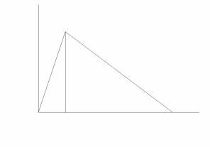
The first part of the amplitude envelope of the earlier mentioned drum sound is named the attack phase and is denoted with the character A. In a drum sound the attack phase will be relatively short. Immediately after the amplitude envelope has reached it’s highest level the amplitude will start to decay. This section is named the decay phase, denoted with the character D. This type of envelope with only an attack and a decay phase is named an AD envelope. Many instruments that are struck like drums or plucked like a harp exhibit this type of envelope.
Figure 1 - AD envelope
To describe an AD envelope it is enough to describe either the angles of the attack and decay slopes or how long the attack and decay phases last. Using time values to describe the attack and decay durations is more convenient and the method used on many different brands of synthesizers. So, an AD envelope of a percussive sound can be sufficiently described by saying that it has an attack time of e.g. 5 milliseconds and a decay time of 1500 milliseconds.
When a note is played on a wind instrument, the amplitude will raise fairly quickly, be stable while the note is sustained and then quickly decay after playing is stopped. There is an extra section between the attack and decay phase. This stable phase is named the hold phase, denoted with the character H. This type of amplitude envelope is named an AHD envelope. The AHD envelope is most common with wind instruments, bowed string instruments and pipe organs. Note that the length of the hold phase depends totally on how long the note is held by the musician, in theory it could hold forever.
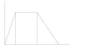
Figure 2 - AHD envelope
With instruments like the piano there are in fact two envelopes that work together to create the final envelope of the sound. The first envelope is defined by the hammer striking the strings and the following vibration of the strings. The second envelope is defined by the interaction between the strings and the sound board and resonance box of the piano. The hammering action has a short attack and a relatively long decay phase and so follows an AD envelope. During this AD envelope the kinetic energy of the vibrating strings is transferred to the sound board and resonance box where this energy builds up strong resonances. The amplitude development of these resonances follows roughly an AHD envelope, the sonic energy lingering in the sound board and resonance box during the hold phase, only starting to decay when the strings are damped when the key is released. The sustain level during the hold phase is lower than the peak level of the AD envelope of the hammering action, as the kinetic energy of the string vibrations also leaks away into the air.
When these two envelopes are joined in one graph it shows an envelope with four phases. In the first phase, when the hammer hits the strings, the overall amplitude will raise quickly and is again named the attack phase or A. Then the amplitude of the hammering action will decay while building up the resonances in the sound board, until it more or less equals the sustain level of the AHD envelope of the vibrating strings/sound board/resonance box combination. This is the decay phase or D. Then the vibrating strings/sound board/resonance box combination will sustain the sound, this phase is named the sustain and denoted with the character S. Finally, when the strings are damped on the release of the key the sound decays quickly, this phase is named the release phase denoted by the character R. This type of envelope is named an ADSR envelope.
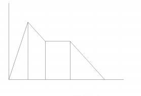
Figure 3 - ADSR envelope
The advantage of an ADSR envelope over an AD envelope is that it allows for the intentional dampening of the sound on a moment chosen by the musician, giving simple and instant control over the note length. The musical difference between the ADSR and the AHD envelope is that the amplitude during the hold phase of the AHD envelope is equal to the maximum amplitude that was reached at the end of the attack phase. In contrast, the sustain level of an ADSR envelope can be significantly lower than the peak of the attack. The ADSR envelope is in fact designed to mimic the mechanics that happen in instruments with a sound board and/or a resonance box. Such an instrument can be seen as having a resonating body and an excitation function, like the piano strings/hammer combination. The excitation function fills up with energy on the moment the sound starts and this energy is then transferred to the resonating body. When a hammering or plucking action is used to initially generate the energy, there is almost instantly a lot of energy available. Then this energy will flow slowly from the excitation function to the resonating body, building up and sustaining the resonance. Right after the attack phase a lot of the released energy will be used to quickly build up the resonance. The decay phase is actually the time needed to build up this resonance. After the resonance is built up only moderate amounts of energy are needed to sustain the resonance, causing only a minor decay in the amplitude level. When the excitation function is stopped, e.g. by dampening the strings in the piano, there is no more energy flow from the excitation function into the resonant body and the resonance will die out rather quickly. This means that the release time is actually the natural reverberation time of the resonant body.
The AD, AHD and ADSR envelopes are well suited to emulate the envelopes of real world percussive instruments, blown and bowed instruments or struck and plucked instruments. But there are many more sounds that have a much more complex amplitude envelope development, a clear example being human speech. To emulate complex amplitude envelopes multi stage envelopes are used. In a multi stage envelope there are several segments that can be increasing, decreasing or stable in level. Two methods are used to describe such an envelope. The first method records the actual amplitude level when the curve changes direction and the time when such a change takes place. The second method records the final amplitude level of a segment and the angle of increase or decrease of the segment, named the rate. When the curve reaches the final level of the current segment it starts to increase or decrease with a new rate to the final level of the next segment. Multi stage envelopes can theoretically have any number of segments, but on most synthesizers they tend to be limited to five or six stages.
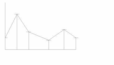
Figure 4 - Multi stage envelope
A modular synthesizer will have modules that can generate an electrical control voltage signal that will exactly follow one of the described envelope curves. Such a module is named an envelope generator. An envelope generator module will have an input that can receive a trigger signal that will start the curve at the beginning of the attack phase. This trigger signal marks the start point of a sound in time. When the trigger input of such an envelope generator is connected to a keyboard key trigger signal, a switch or a drum pad the musician can instantly start the envelope. But the trigger signal used to start the envelope can also originate from a module that can generate a train of trigger pulses in some rhythm or from a computer, or any other device that can generate a compatible trigger signal. By itself an envelope generator will do nothing, it always needs a trigger signal as a command to start the envelope. And when the envelope has fully decayed it will meekly wait doing nothing, until another trigger command is given.
On a instrument each note has a distinct pitch. The pitch depends on how many vibrations per second are present in the played note. The number of vibrations per second is named the frequency. In other words, frequency is how many occurrences of repeating vibrations or cycles of a certain waveform happen during a second of time. Frequency is expressed in Hertz or Hz. These days it is custom to tune instruments to the note A that has a frequency of 440 Hz, meaning that this note makes the air pressure vibrate at a rate of 440 times a second. The lowest number of air pressure vibrations the average human ear can pick up has a frequency of about 20 Hz. The highest number can be as high as 20.000 vibrations per second, a frequency of 20 kHz (kilo Hertz).
Like electrical devices internally deal with amplitude they also deal with frequency, while pitch deals more with how the human mind perceives frequencies. Notably frequency differences between the notes on musical scales. A note with a frequency that is twice as high as the frequency of another note will sound twice as high. E.g. a note at 440 Hz will sound twice as high as a note at 220 Hz. This is interval is named an octave. A note with a frequency which is three times as high, so at 660 Hz, will not sound two octaves, but only ‘one octave and a fifth’ higher. The note that will sound two octaves higher as the 220 Hz note will in fact have a frequency of 880 Hz, meaning that this frequency, which is perceived ‘three times as high’ as the 220 Hz frequency note, has an actual frequency value that is four times higher. And a note that sounds four times higher will have an actual frequency of 1760 Hz, which is eight times higher. The explanation is that a note that sounds exactly one octave higher must have it’s actual frequency value doubled. Look at the frequency values for all A notes over an eight octaves range:
55 Hz - 110 Hz - 220 Hz - 440 Hz - 880 Hz - 1760 Hz - 3520 Hz - 7040 Hz
This shows that the relation between the notes on the well tempered twelve note musical scale and their actual frequency values is exponential. This is very important to realize, as it might lead to confusion. On modular synthesizers pitches can be controlled either through their corresponding notes on the exponential musical scale, or through the exact frequency values on a linear frequency scale. Only few modular systems offer both methods. For musicians wanting to play in the western well tempered twelve note scale the exponential method is the most convenient, as it translates directly to the black and white keys on a keyboard. This method is also named the Volt/Octave norm. But for sound synthesis the linear method has some very useful features. Meaning that for the more experimental composers and sound designer artists this linear method, also named the Volt/Hertz norm, might have interesting advantages.
Some musical instruments can only produce one note at a time, these instruments are named monophonic instruments. Examples are the silver flute, the trumpet, etc. Other instruments allow for many notes to be played at the same time, like the piano, the organ, etc. These are the polyphonic instruments. Polyphonic instruments can play both single notes and chords. A chord is a layering of several notes in a certain musically pleasing relation. One of the pitches in the chord can appear to dominate over the others. This note is named the key or root of the chord. The other pitches have relatively easy frequency ratios with this root pitch. These frequency ratio’s might be 3:2, 4:3, 5:3, 5:4, etc.
In the more experimental electronic music genres chords with more complex and exotic ratio’s than those used in traditional western music are often used to create rich sounding sonic textures. To avoid confusion with the traditional chords and their traditional names it is better to use the name composite sounds for these sonic textures. These textures are often used in experimental electronic music, soundscapes, drone music, film music, etc. In these musical genres it might be the changes in timbres that define the development of the composition. Melody, harmony and rhythm are made subordinate to these timbral developments. E.g. rhythm might be created by rhythmic changes in timbre. Composers have the freedom to work out their own personal system of composing and sound synthesis can be an important part of that system. There is a choice of synthesis systems and material can be intuitively assembled ‘by ear’. Without doubt it takes a lot of experience with sound synthesis to make such efforts musically worthwhile.
Traditional music notation is not very useful for the compositions that involves the notation of the development of the sonic developments in the sound synthesis. Pitches and tuning can be freely defined and are difficult to express in traditional notation. many contemporary composers have experimented with new ways of notation and the resulting scores sometimes look more like paintings than like a traditional score.
The frequencies of some of the partials in a single pitched sound might coincide with the intervals found in the traditional chords. E.g. an interval of an octave and a fifth is related with the third harmonic, making a fifth also related to that third harmonic, as it happens that the second harmonic of a fifth will coincide with the third harmonic of the root. But a monophonic sound can have something like up to a hundred harmonics present within the hearing range. And there are many possible relations that can not be simply expressed by chord intervals. To define the relation between a root frequency and a second frequency the frequency ratio is used. This ratio can be expressed in a fractional number containing a numerator and a denominator, notated like n:d. When the ratio is 3:2 then the second frequency is 3/2 or 1.5 times higher. This system was already used in ancient cultures to define musical scales, an well known example is the Pythagorean scale.
The harmonics of a fundamental frequency always have a ratio of n:1, where n can be any positive integer number. Partials do not necessarily need to have a simple ratio to the fundamental, many drum sounds are good examples. These are sounds that can have non harmonic partials present, which still melt nicely into the overall drum sound.
Chords sound best in just tuning, in just tuning exact and simple ratio’s are used to define the scale. Many synthesizers offer the possibility to use both well tempered scales with a user definable amount of notes in an octave and a number of just tuning scales.
On a traditional keyboard the keys for the notes in a chord need to be played at once. Modular synthesizers offer features to ‘preprogram’ chords and composite sounds under single keys. Defining different composite sounds which are tuned to exact ratio’s under different keys, allows for the play of complete soundscapes in just tuning.
When the amount of partials is increased and several non harmonic partials are added the sense of pitch might be lost. Formally the sound becomes noise, but noise can have an infinite amount of different timbres. And sounds that are definitely noise can generate a sense of pitch, like the whistling of the wind.
A sound can have a single pitch, be with or without harmonic or non harmonic partials, be the layering of some pitches like a chord, a composite sound, a complete soundscape and finally up to completely pitchless like the sound of ocean waves. While the sound sounds the pitch or pitches can glide, vibrate or jump. This is named the pitch envelope. It is important to have very precise control over the pitch envelope, as unlike the amplitude envelope the pitch envelope doesn’t follow simple graphs. It is best to bend the pitch by hand, to give the sound the right intonation. A device named a pitch bender allows for expressive manual control. Most common pitch benders are the pitchbend wheel, the pitch stick and the ribbon controller.
Timbre is the sonic quality of a sound that defines the distinct character of this particular sound and makes it recognizable amongst other sounds. When a trumpet player and a violin player play the same note with exactly the same loudness contour and pitch bend, the difference in timbre is still clear and hardly anyone will have a problem in recognizing the sound of the trumpet from the sound of the violin. But there is more than recognition to a timbre, there are additional musical properties to the timbre of a particular sound. These properties are often very subjective. Vague names are used to classify their sonic effect, like a timbre can be damp or bright, muddy or squelchy, woody or metallic, singular voiced or chorused, thin or fat, massive and impressive, soft or aggressive, warm or cold, deep and spaced or right into the face, etc. But before these kinds of subjective qualifications can be dealt with there must be an understanding on how the basic timbre of a sound comes about. In sound synthesis there are a number of different techniques to create certain timbres. The simplest technique is to make a digital recording of a sound of a particular instrument, commonly named a sound sample. The sound sample can be played back at a different pitch and one of the first things one notices is that the timbre changes in an unnatural way when the sample is played back only just a few notes higher or lower. And when the detuning is more than an octave the sound is hardly recognizable any more. This means that there is no simple relation between the pitch and loudness contour and the timbre of the sound of an acoustic instrument. In general the overall loudness contour is the same for each pitch, although initial segments of the loudness contour, like the initial attack and decay phase, might be shorter for higher pitches. When playing different notes on an acoustic instrument much more complex things seem to happen. For one there are some fixed frequency ranges that seem to be present in all notes and the relative strength of these ranges seem remain pretty constant no matter how much the pitch changes. Instead these frequency bands seem to be much more influenced by how loud the note is played, a good example is a muted trumpet. Additionally the playing style of the instrument can change the timbre in sometimes dramatic ways. This means that timbre can not be captured with one single parameter, like the frequency parameter or the amplitude parameter. In fact, there are many parameters that define the timbre of a sound. So, while a sound still has the three basic parameters loudness, pitch and timbre, the loudness on a certain moment can be defined by only one amplitude value, the pitch can be defined by one or more values, e.g. for a chord there might be three frequency values, while for timbre there might be a whole array of values needed to describe the sound. So, what was named up to now a basic parameter of sound is not simply one single value, but in practice a collection of values, used together to define a generalized parameter like ‘a trumpet sound’.
To gain some more insight it often pays to simplify the situation into a simple model. A very useful model for acoustic instruments is the exciter/resonator model. In this model the instrument is roughly divided into two parts and the interaction of these two parts with each other is responsible for the resulting timbre of the instrument. This model is able to describe in a simplified way what happens in most acoustic instruments. A very good example is an acoustic guitar, where a string is used to make the body of the guitar vibrate. The string acts as the exciter and the guitar body resonance box as the resonator. The sound of only the string itself is not loud enough to be musically useful and the resonance box is used to amplify the sound. Additionally, the resonance box shapes the timbre of the sound. This model immediately explains why a sampled sound starts to sound unnatural when detuned to a new pitch, as the resonant guitar body does not change for a new pitch. So, the timbre for each note in a real world instrument is defined by how the resonant body or resonator interacts with an excitation at a certain pitch.
The traditional analog synthesizer tries to simulate this exciter/resonator model by using two separate modules that act as an excitation function and a resonator. For the excitation function an electronic sound source, named an oscillator, is used. The oscillator module is similar to the strings, reeds, etc., of acoustic instruments In its effect an oscillator provides a train of steadily repeating pulses on its output, the number of pulses per second defining the frequency. A single pulse is named a cycle and the cycle can have various forms, named the waveform. The resonating body is simulated by the use of various types of resonating filters. The sonic energy in the signal from the oscillator cannot leak away in the air in the form of sound or warmth like in an acoustic instrument, instead the flow of sonic energy is continuous when the oscillator is connected directly to the filter. As a result a synthesizer can create steady pitches with resonance effects that can sound forever. In order to create natural swells and decays an extra set of controllable amplifiers must be used to control the overall volume development of the sound. These amplifiers can be controlled by devices that generate a control signal which follows the envelope curves as described in a previous chapter. When designing sounds it is useful not only to think in electrical signals that flow from module to module, but also in terms of sonic energy that excites another module, where the energy is ‘transformed’ into timbre. Like how the sonic energy from the oscillator is actually exciting the filter in a similar way as a guitar string is exciting the body of the guitar.
When the exciter/resonator model is patched on a modular synthesizer, there are three modules chained in a serial way, meaning that their respective outputs will go into the input of the next module in the chain. The first module is the oscillator and its output goes into the input of the second module, the filter. Then the output of the filter goes into a third module, a controllable amplifier which is responsible for the volume envelope. The general notion is that in this model the oscillator module defines the pitch parameter, the filter defines the timbre parameter and the controllable amplifier defines the amplitude parameter. This is almost true, as the timbre parameter is actually defined by how the filter reacts on the oscillator, as in fact the timbre is created by the cooperation between the oscillator and the filter. Different waveforms for the cycles of the oscillator will excite the same filter in different ways, creating different sonic effects. So instead, one can think in terms of how the exciter/oscillator is exciting the resonator/filter and the stream of continuous sound this process creates is controlled in amplitude by the controllable amplifier. Later on in this book the advantage of thinking in this more correct way will become clear when looking at the synthesis of certain sounds in more practical detail.
The three modules, oscillator, filter and controllable amplifier, each get their own separate control signals to be able to dynamically shape the sound. A module can receive more than one control signal, e.g. the oscillator can receive a control signal defining the pitch of the note it has to play, but additionally receive an extra, slowly varying, control signal to give a vibrato effect to the pitch. On the analog systems of the past, where the control signals were actually voltage levels, the modules were named Voltage Controlled Oscillator, Voltage Controlled Filter and Voltage Controlled Amplifier, abbreviated to VCO, VCF and VCA. Which is why this model is still referred to as the VCO-VCF-VCA model, although digital system do not work with discrete voltage levels anymore.
Picture of the schematic!!!
The basic VCO-VCF-VCA patch has the advantage that it can mimic the dynamics that happen in an acoustic instrument through the control inputs on the modules. But it is in fact very hard to convincingly imitate an existing acoustic instrument with the model. In general the synthesizer is not really very interesting to imitate existing instruments, instead it is mostly used to create totally new musical sounds, that can be played with the same sort of dynamics and sonic characteristics of a certain acoustic instrument. Playing style is very important here, e.g. when a synthesized sound that very vaguely reminds of a flute is played with a flute-like playing style, the human mind will have the impression of a flute, though maybe a cheap flute. But when a very close imitation of a flute sound is synthesized and played in a polyphonic way like an organ is played, it will sound much more like an organ that like a flute. It is very important to realize that playing style is as important as synthesizing a certain timbre to create the effect of a certain existing instrument.
In the music industry there is a commercial need for convincing electronic imitations of real world acoustic musical instruments. When in a recording studio a string section has to be recorded, it is much cheaper to use an electronic instrument than to hire a couple of musicians for a few days. Since the early seventies studio’s tried to use VCO-VCF-VCA model synthesizers to replace real musicians. This led to a common but false believe that the main purpose of these synthesizers is to imitate existing instruments. In fact, imitation is their weakest point. It is a much healthier approach to see a synthesizer as an instrument by itself, with its own musical right of existence and use it as such. In the eighties samplers replaced the original VCO-VCF-VCA model synthesizers in the studio, as when using the right set of samples, samplers are much more convincing in imitating acoustic instruments. Just think about digital piano’s, these are in fact preprogrammed samplers with in general several samples for every single key. For recording purposes these digital piano’s do perform very well. Still, samplers lack the kind of dynamic timbral control that the VCO-VCF-VCA model synthesizers have. So, when it is about imitating acoustic instruments, samplers have the realism in the timbre, but lack the dynamics. In contrast, the VCO-VCF-VCA model has the dynamics, but in general lacks realism in the timbre of imitated acoustic instruments.
To overcome the limitations of both the sampler and the VCO-VCF-VCA model, there have been attempts to use methods that try to directly synthesize the audio signal of the timbre without using resonant filters. In these techniques only oscillators are used, but special types with a dynamically controllable variable waveform. While the sound develops, the waveform is dynamically reshaped in a way that the resulting timbre follows the timbral development of the instrument to be imitated as close as possible. This technique is named waveshaping. Waveshaping takes a basic waveform and then distorts this waveform by a distortion function. There are two subclasses of waveshaping techniques. Techniques in the first class distort the amplitude of the waveform at audio rates, techniques in the other class distort the frequency of the waveform, also at audio rate. To understand the difference and realize why there are only two subclasses, note that any momentary waveform can be drawn as a two dimensional graph on a piece of paper. When doing so it becomes instantly clear that there can be a distortion in the vertical direction, which is the amplitude value, or a distortion in the horizontal direction, which is the time axis. And time of course relates to frequency. Distortions in these two possible directions are named amplitude modulation in the audio range or AM and frequency modulation in the audio range or FM. A variation on FM is where it is not the actual frequency parameter that is heavily modulated with an audio rate signal, but instead the phase of the waveform is modulated. This is properly named phase modulation or PM. PM is a ‘digital only’ technique and offers a small advantage over FM as it allows for feedback modulation or self modulation of the waveform oscillator without altering the pitch of the signal. For the rest everything that applies to FM also applies to PM. When AM, FM or PM techniques are used in a synthesizer the basis is in general a digital sinewave oscillator. Some types of waveshaping synthesizers, like the Yamaha DX-type synthesizers, use only the phase modulation technique and are commonly (but wrongly) named FM synthesizers. On the better traditional analog modular synthesizers both AM and FM is possible, but the frequency stability of the analog oscillators is not enough to precisely use the technique to do convincing imitations. A digital modular synthesizer like the Nord Modular G2 is able to do AM, FM and PM waveshaping and also combine these techniques together to create expressive timbral developments in a straightforward and intuitive way. Additionally, on the G2 resonating filters can be inserted in the modulation path to patch models with very powerful sonic characteristics.
One drawback of the waveshaping techniques is that, when imitation is the goal, complex mathematics is involved in calculating the exact depths of modulation to create the wanted timbral developments of certain sounds. With the AM technique this involves Chebyshev functions and the FM technique involves Bessel functions. Interestingly the commercially most successful synthesizer up to now, the Yamaha DX7, uses the PM technique. Still, programming sounds on the DX7 was very difficult, only very few people had any notion on how to go about. Luckily the DX7 came with a useful set of factory preset sounds, and the commercial success of the DX7 has more to do with the fact that it came at the right moment in time and with the right amount of polyphony and the right size, weight and price. The complex DX synthesis method with its six phase modulatable sinewave oscillators per voice was happily ignored by the average musician.
One important notion is that waveshaping using AM and FM techniques relate to each other in a very close way. One might be tempted to think that amplitude modulation cannot change the pitch, but in fact amplitude modulation of certain waveforms by other certain waveforms can actually create a fixed detuning of the pitch. Just like frequency modulation can keep the pitch fixed while only affecting the timbre of the sound. So, both are really related. But it goes way beyond the purpose of this book to go deep into the basically mathematical subject of proving this relation in a scientific way. Later on in this book there will be some simple practical recipes to use these properties of AM, FM and PM to create various musically interesting sonic effects.
In practice there is one important difference between AM and FM. AM can always be done after the output of the oscillator with a controllable amplifier module, there need not be a specific input or function on the oscillator to be able to use AM. The controllable amplifier however must be able to accept bipolar input signals. A standard VCA module has a bipolar input for the audio signal, but the input for the amplitude level is unipolar. Whenever the control signal on this input becomes a negative value the VCA simply shuts off. However, when a module named a ringmodulator is present on the system, this module can be put to good use instead of a VCA, as this ringmodulator is technically a bipolar controllable amplifier that can handle both positive and negative signals on both its inputs. When a lot of ringmodulator modules plus additional mixer modules are available, Chebyshev functions can be patched to do the timbral shaping, using one single sinewave as the initial waveform.
When using the FM technique for waveshaping purposes a special FM input on the oscillator is needed. This FM input must be able to control the frequency in a linear fashion, the standard pitch input with its exponential V/Oct control curve is less useful, as it will quickly detune the pitch.
The difference in timbre between acoustic instruments depends on a lot of factors, for instance the dimensions and materials of the instrument body and whether it uses strings, skins, reeds, etc. to be excited. Even ambient temperature, air pressure and dampness of the air can have an influence on the timbre. Additionally, variations in playing style can create different timbres from the same instrument. And as there are so many different types of acoustic instruments, it is hard to generalize on how their timbres are created. The resonant body can be a fife, like with a flute, where it is air that resonates within its cavity. It can also be a wooden resonant box or metal can that can resonate along with strings or skins. It can be a sound board that resonates or a sound board mounted in a resonance box. Some instruments have more than one resonance box, like some ethnic string instruments. Some resonance boxes are real boxes, like a guitar, or they may be pipes that are mounted close to the part of the instrument that functions as the exciter, like with a vibraphone. So, resonators can take on many forms and be made of different materials, but the generalized purpose of the resonator is to sustain the sound and give the sound its main timbral character. In practise, most of the sound which is actually heard from an acoustic instrument is radiated from the resonant body. To get into resonance the resonant body needs to be excited by some sort of excitation function. This can be the plucking, bowing or hammering of a string, the beating on a skin or a strip of metal or wood, a reed, the air pressure of a flow of air, etc.
As an example let’s have a look at a plucked string instrument like the guitar again, it has a resonant body plus one or more strings mounted in a way that the strings can swing free, while one side of the strings rest on a bridge. The bridge is the path through which the kinetic energy in the swing of the string can be transferred to the resonant body. The kinetic energy will start to travel through the resonant body in the form of waves, which get reflected at the sides of the resonance box. Depending on the form and dimensions of the resonance box the waves and their reflections will form interfering wave patterns with knots at certain locations on the surface of the box. These knots add to the formation of formants, which are small frequency bands at fixed positions in the sound spectrum where frequencies get strongly emphasised. Imagine that the kinetic energy, which flows from the string, gets moulded into a typical timbre with strong resonances at certain fixed frequencies. When the frequency bands where these resonances occur are narrow and have a strong resonance, they will add more to the pronounced character of the timbre of the instrument.
Musically important formants are found in the frequency range that lies roughly between 500 Hz and 3500 Hz. E.g. human speech is based on how three to five strong formants shift from place to place in this range over short amounts of time. The formants that are present in the sound will melt together into one timbre and the relation between these formants is named the formant structure. In other words the formant structure is the total of the formants present in the sound and how the formants relate to each other. The individual formants can hardly be heard, as the human mind uses the total formant structure to recognize sounds. The basic technique used in sound design is to create sounds with expressively controllable formant structures. When using a synthesizer, very expressive and characteristic timbres can be created by causing strong and dynamically moving formants in the 500 Hz to 3500 Hz range.
Instruments like the grand piano have a sound board which is mounted in a resonance box. The kinetic energy first travels from the strings to the sound board and then from the sound board to the resonance box. Strings, board and box together form the mechanics which are responsible for the final basic timbre. The heavy sound board and thick and tight strings of the grand piano can store a lot of energy. This is one of the main reasons why the grand piano can play relatively loud compared to other instruments. E.g. plucked and bowed instruments like the guitar and the violin sound less loud, as their resonance box is made of relatively light and flexible material. In the case of a flute the fife itself is the resonator, and the prime resonance frequency of the fife will define the pitch of the sound. There needs to be a constant flow of air into the fife to sustain the vibration at the resonance frequency. When the air pressure increases by overblowing the flute there will be more turbulence in the air flow and this can create resonances at higher harmonic frequencies.
To summarize, almost every acoustic instrument or sounding object can be assumed to be a resonant body that is excited in some way, the excitation causing the resonant body to vibrate and resonate on the body’s natural resonance frequencies. The resonance frequencies together form a formant structure that is mainly responsible for the final timbre. Energy is fed into the resonant body, which transforms the energy into a timbre with a specific formant structure. Most of the transformed energy leaks away into the air while the rest is transformed into warmth. This assures that the sound of an acoustic instrument or object will always die out when the excitation function stops and no more energy is fed into the resonant body. The shape of the resonating part of the instrument will add significantly to the final timbre of the instrument, a reason why acoustic instruments have their particular appearance.
As synthesizers are in practice often used to emulate existing instruments, recognition is the keyword when trying to emulate such a sound. The sound doesn’t have to sound exactly like its real world counterpart, as long as people recognize it as sounding like that instrument. The trick is to make the mind of the listener associate the synthesized sound with the sound of the real world instrument. When the sound has the right sort of timbre and it is also played in the playing style of the real instrument the association is quickly made. As said earlier, playing style is very important here, and playing style can include playing the timbre. An example is how a trumpet player can drastically modulate the timbre by muting the trumpet with a beaker. Using a certain playing style can apply for totally new synthesized sounds as well. When a sound is created which is not modelled after an existing real world sound it often pays to experiment with different playing styles, until a style is found that seems to suit the sound best.
Changing formants can be very important in expressively playing the timbre, a well known example is the effect of the Wah pedal as used by electric guitar players. The wah effect is created by introducing a strong formant in the timbre, which is swept through the audio spectrum by a foot pedal. The popularity of the Wah pedal amongst guitar players has to do with the fact that with only a single controller, the foot pedal, the timbre of the sound can be expressively shaped. The guitar player can still do everything to pitch and amplitude with his hands, but now he has his foot as an extra way to express himself through tonal shaping of the timbre. For controlling a keyboard synthesizer two hands, and optionally feet, can be used. On the first monophonic synthesizers from the seventies the melodies could be played with the right hand, leaving the left hand to expressively play the timbre. One or two modulation controllers mounted to the left of the keyboard could be used to either bend the pitch, add some vibrato or sweep the timbre. When the modulation controller is a modulation wheel, it can control one single parameter in a sound. Another popular controller from the seventies is the joystick or X-Y controller, which allows for two parameters to be played by one hand. E.g. by letting the joystick sweep two independent formants or resonance peaks, expressive talkative timbre modulations can be played. Another possibility of the joystick is to crossfade between a maximum of four distinct formant structures.
Playing the timbre with polyphonic synthesizers is a bit more difficult, as on such an instrument the melodies are generally played by both hands. When the keys on the polyphonic keyboard are velocity sensitive, the velocity value can be used to control the timbre. However, the velocity value is sampled when the key is hit and keeps constant for the duration of the note. For this reason some of the better polyphonic synthesizers are fitted with an aftertouch sensitive keyboard. After a key is hit the timbre can be modulated by pressing harder on the pressed keys. Aftertouch can replace the modulation wheel effect, but it needs a lot of practising to learn to play it well. Some polyphonic synthesizers are equipped with a connection for a breath controller. This is a little tube that can be worn on the head like a headset, with the end of the tube right before the mouth. By blowing into the tube the air pressure is converted into a control signal that can be used to play the amplitude and/or timbre of the sound. And almost all polyphonic synthesizers are equipped with a connection for at least one foot pedal. Still, modern synthesis techniques allow for an enormous degree of controllability and the traditional human interfaces like the above mentioned controllers are not up to unleash the true sonic potential of the present day modular synthesizers. There have been many experiments with new controllers, like gloves with bend sensors, distance detectors like Theremin antenna’s or infrared light distance sensors and all other available types of sensors. But no matter how well the sensors and interfaces work, they all require to learn a new playing style to play the sensors in a musical way.
The basic architectur of a modern synthesizer can be subdivided in three parts, the human interface to play the instrument, the sound engine that houses all the modules and does all the synthesis work, and some intelligence in between that connects the two parts in a sensible way. The intelligence part is housed in the microprocessor that has been present in polyphonic synthesizers since the end of the seventies. Many times this is the same processor that also processes MIDI information received form another instrument or play controller. Over the years these processors have become very powerful, today it is really like there is a small computer present. One of the newer functions that makes use of this extra power is the possibility to use a single physical controller to control several control signals or values at the same time in an intelligent way. This allows for modulation of the timbre over a range from very subtle to very complex. This technique is named morphing. In essence morphing does a crossfade between a number of knob settings to a new set of knob settings, the knobs that participate in the crossfade are named a morphing group. Morphing allows one hand to simply and intuitively play very expressive timbral modulations.
The timbre of a single pitched sound with a static amplitude and a static timbre can be analysed into a harmonic spectrum plot. Such a plot reveals graphically all the partials present in a single pitched sound, and it is a useful means to analyse or define a static waveform from an oscillator sound source. The maths used in the analysis actually assumes the data to be a single cycle of a waveform to produce meaningful results.
In the nineteenth century it was discovered that all sounds are in fact the addition of a number of sine waves at different frequency and amplitude values. When the sound has a single pitch these sine waves will have a simple harmonic relationship to each other.
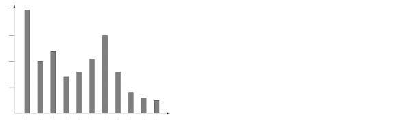
Figure 5 – Example of a harmonic spectrum plot
The sinewave with the same frequency as the perceived pitch of the sound is named the fundamental or first harmonic. All other sine waves present in the waveform have a frequency value that is an exact multiple of the frequency of the fundamental, the second harmonic will be two times higher in frequency, the third harmonic three times, etc. The group of all possible harmonics with their individual amplitudes is named the harmonic series. A harmonic will always have a harmonic relationship with the fundamental, but there might be components in the sound that do not have this harmonic relation. Then the name partial is used, as a partial does not necessarily need to have a harmonic relation, like the harmonics do.
In appearance a harmonic spectrum is a plot that on the horizontal axis shows the numbers for the harmonics. There is a vertical bar at each harmonic number position, which shows the amplitude on the vertical axis scale for the corresponding harmonic. The horizontal axis has a linear subdivision in whole numbers from the number one for the fundamental to a theoretically infinite number. The frequency of the nth harmonic in the plot has a frequency ratio of n:1 to the fundamental frequency. In practise it suffices to plot only the first fifty to hundred harmonics, as higher harmonics might very well be above the highest frequency of the human hearing range. The amplitude values of the vertical bars are in general percentages, not absolute values. The harmonic with the strongest amplitude is normalized to 100% and the amplitude values for all other harmonics are scaled to percentages between 0% and 100%. The relation or ratio between the amplitudes of the harmonics defines the timbre of the sound. The plot shows no absolute frequency values for the harmonics, but to get absolute values the frequency of every harmonic can be easily calculated by multiplying its number by the actual frequency of the fundamental. The amplitudes are calculated by first defining an absolute amplitude value for 100% and then calculating the amplitude values for each harmonic by scaling them to their respective percentages.
In the simplified exciter/ resonator model that was used earlier to describe the mechanics of acoustic instruments, the harmonic spectrum can be used to define the spectrum of a continuous excitation function. However, the harmonic spectrum is always a snapshot at a certain moment in time. In the real world the harmonic spectrum of an excitation function will vary over time, depending much on playing style and modulations applied by the musician. E.g. when the harmonic spectrum of a reed is analysed, it will show that it changes by the air pressure that is exercised and by the position and pressure of the lips on the reed. Morphing between two or three harmonic spectra allows for a more expressively playable excitation function. By using e.g. a breath controller assigned to a morph group it is possible to morph between two spectra, while an X-Y controller can morph between up to four spectra.
In scientific research papers harmonic spectra are generally plotted a bit different, as they might express not only sine but also cosine components. With such plots additional phase relations between harmonics can be analysed. But the why goes beyond the practical purpose of this book.
Next to a harmonic spectrum a spectrum plot of the total human hearing range can be drawn. Such a graph is named a sound spectrum plot. The horizontal axis will show absolute frequency values. As there is an exponential relation between the octaves and frequencies the horizontal axis has in general a logarithmic scale. When the harmonics of a sound of a certain fundamental frequency are plotted as bars the plot will become denser to the right.
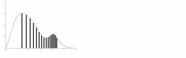
Figure 6 – Sound spectrum showing a harmonic series
The sound spectrum can also show partials that do not have a harmonic relation, show chords or show the sound spectrum of a very complex sound. There will be a bar for every sinewave component that is present in the sound. It is difficult to exactly read values of bars in such a plot, and in general it is not meant to be exact, but instead to give an impression of the overall sound spectrum. By connecting the tops of the bars a curve can be drawn that estimates the current sound spectrum. Such a curve is named the spectral envelope. The spectral envelope is in general used to get an idea of the sonic power that is present in a certain frequency band of interest.
The harmonic spectra for notes with different pitches can differ significantly on an acoustic instrument. By analysing the harmonic spectra of all notes and plotting them in a sound spectrum, a plot is generated that on the horizontal axis reveals the places where resonances or formants occur. Such a plot can reveal the formant structure of an instrument and can be very helpful in designing a sound that closely resembles the instrument. Such a plot is named a formant spectrum and is plotted as a spectral envelope on a logarithmically scaled horizontal axis. In appearance it looks just like a sound spectrum plot, but it has no bars, only the spectral envelope. The difference is subtle, a sound spectrum plot shows an analysis of an existing sound, while a formant spectrum plot shows which formant areas are needed to create a sound that is not yet in existence. A formant spectrum plot is an important piece of information for a sound designer.
In the exciter/resonator model the formant spectrum plot can describe the effect that the resonant body has on the sound signal that comes from the excitation function. It shows the frequency ranges which are boosted and ranges which are attenuated. There might be small strong peaks, indicating a very strong resonance, and small dips or notches where a frequency is strongly attenuated.
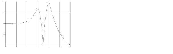
Figure 7 – Formant spectrum with two formants and a notch
The reflections of the waves that travel through a resonant body will cross waves that travel in other directions, causing an interference patterns similar to the interference patterns when some stones are thrown in a small pond. Sometimes a wave of a certain frequency will be cancelled completely by its own reflections and at that frequency there will be a notch in the formant spectrum. But another frequency might be amplified by its own reflections and this will show as a resonance peak or formant in the plot.
A formant spectrum is relatively static, but slight variations might occur depending on how strongly the resonant body is excited. Formants will hardly shift place but some might broaden or become more emphasised. Being able to morph between somewhat more complex formant spectra is an interesting option in sound synthesis, but in practice this needs special complex filters that are hardly found on synthesizers. Instead, on analog synthesizers level dependent distortions based on non linear characteristics of certain electronic components, aptly named distortion, are commonly used to emphasize sonic differences between soft and loud notes. When tweaked subtly, this technique can in practise work out very well. Digital techniques offer the possibility to use mathematical functions or lookup tables to describe level dependent operations that mimic the effects that can happen when the resonator gets excited by different levels of energy.
When the effect of a filter is described the same sort of plot can be drawn. Although in research papers you might find a different way to accurately describe the effect of filters, named the impulse response. The impulse response is the signal that will be on the output of the filter shortly after the filter input has received a single pulse of infinite short duration and with an infinite amount of energy. In practice a very short spiky pulse is used, with the maximum signal level the device can handle. When the signal on the output is sampled and analysed in a plot it should then reveal the formant spectrum of the filter. A similar method can be used to analyse the reverberant characteristics of a space like a concert hall, which in a way is an enormous resonant cavity. To produce the impulse a hydrogen implosion is used. A little bit of hydrogen gas is led by a small tube into some soapy water, forming a little bubble of hydrogen gas at the surface of the soapy water. The hydrogen is ignited by pushing a burning matchstick into the bubble, causing the bubble to implode. Such an implosion creates an almost ideal pulse. The sound wave of the pulse reflects against the walls and all the reflected waves form interference patterns in the space, colouring the sound of the reverberation of the pulse. This describes nicely what the impulse response actually is, in this case the literal reverberation of the space right after the hydrogen implosion. The analysis of the recorded impulse response can be used to program an huge electronic multi-tapped delay line, that will then give a very close simulation of the reverberation effect of the analysed space.
When a formant spectrum plot is specifically used to describe the effect that an electronic device like a filter or distortion function, a resonance box or a reverberating space has on a sound, then scientists name the plot the spectral transfer function of the effect. This is the graph that shows how the sound spectrum is changed by the effect. This transfer function is all important as it describes exactly what will happen to any frequency component in the original signal or sound. When working with synthesizers musicians use names of several typical transfer functions almost unconsciously. Like when they insert a lowpass filter or a highpass filter in a signal chain the lowpass or highpass refers to the type of transfer function of the filter.
Devices like microphones and loudspeaker boxes also have a transfer function. For these devices two transfer functions can be plotted, one that reveals how frequencies are affected and another that shows the phase shift or time delay for each frequency. These phase shifts or time delays are caused by the reflections of sound waves within the loudspeaker cabinet and the placement of the loudspeakers that have to reproduce the different frequency bands. A set of loudspeaker boxes that have a flat frequency response, but a wildly varying phase response, might faithfully reproduce a single monophonic sound, but will probably totally mess up the original stereo field for a stereophonic sound. So, note that a loudspeaker box in itself is also a resonant box and can significantly influence the colour and the spatial character of the reproduced sound. Ideally, both the transfer function plots for microphones and loudspeakers should show a flat horizontal line, which would mean a perfect device. But in practice microphones and loudspeaker boxes are far from perfect, meaning that coloration of the sound is inherent. That doesn’t need to be a problem, as this coloration might very well be a wanted feature. Just think of an electric guitar amplifier and accompanying loudspeaker cabinet. In this case the cabinet actually takes over the function of the absent resonance box on the electric guitar. A strong coloration of the sound by the cabinet is very important here. For doing different kinds of sound recordings, a typical music recording studio will have several types and brands of microphones available. A microphone used to record vocals will most probably never be used to record a drumkit, unless maybe a special effect in the recording is wanted. The art of recording is very much about picking a microphone that gives the right sort of coloration for the timbre, and at the sound level produced by what needs to be recorded. Of course plots of transfer functions are really of little use here, a good set of ears and a lot of experience is much more helpful. As in the end the only rule is that it has to sound right.
To analyse how a timbre develops over time requires to go another step further with the plot. An example of sound with a very complex and dynamic timbral development is human speech. The human vocal tract is actually a very complex filter where several formants are created in different places of the vocal tract. Additionally the vocal tract can modulate some of these formants to create effects like e.g. growling sounds. Each individual’s vocal tract has slightly different dimensions and several muscles are involved to shape the vocal tract. All these muscles can have their own individual tremors, causing their own different modulation effects. There is an unlimited amount of subtle sonic effects possible, giving each individual his or her individual voice. When thinking about this, it is pretty miraculous that humans can instantly recognize the voices of an enormous amount of individuals. The reason for a musician to use a modular synthesizer is many times to create his or her own individual sound, a sound that clearly stands out against the sounds used by other people. Such a sound needs character, and then it is good to realize that a good example of sounds that definitely have character are vocal sounds. So, when there is some basic understanding of the mechanism of vocal sounds, it is probably easier to create individual sounds with a definite personal character. Regrettably, human sound is a very complex matter, up to this day synthesized human speech still does not sound very natural, though recent technologies do come very close. The main clue to create individual synthesized sounds is to realize how formants play an important role in vocal sound. Human speech researchers divide human speech into phonemes, the short sounds that from the characters of speech. A phoneme has definite timbral development which cannot be analysed with a single formant spectrum plot. A formant spectrum of a phoneme can have up to maybe twenty five formant peaks or notches which are continuously altered, shifted and modulated while text is spoken. Additionally it might be voiced or unvoiced, meaning that there is either a definite pitch or more a noisy character without a detectable pitch. To be able to plot such sounds the sound is split into very short parts and for each part an analysis is made. These analyses are then plotted glues to each other in a special way, each individual analysis is plotted in a straight vertical line where the vertical position is the frequency axis. When a certain frequency component is present it is plotted by a grey dot, the dot becoming darker when the amplitude is stronger. The vertical lines are put next to each other to result in an image showing grey wavy patterns. The image is named a sonogram and reveals how the formant areas in a sound develop in time. The sonogram must be interpreted from left to right. Here are two examples of sonograms.
Figure 8 – Sonogram of an upward sweeping saw tooth waveform
The sonogram in illustration Figure 8 shows the analysis of a saw tooth wave sound that is swept up in pitch. Each grey line shows a harmonic, the lowest line being the fundamental. It is not difficult to imagine what happens in this sound.
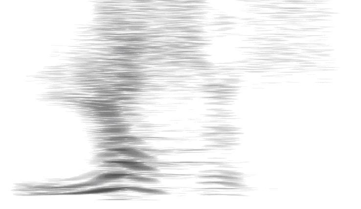
Figure 9 - Sonogram of the Dutch word 'jasses'
The sonogram in illustration Figure 9 is the analysis of a Dutch word ‘jasses’, as spoken with much expression by the late Dutch poet Johnny van Doorn. The word expresses a strong feeling of disgust, like when one expects to drink a good wine but it has turned into vinegar. The initial unvoiced ‘j’ is shown in the lower left corner and very quickly morphs into the ‘àh’ when the two distinct dark lines start. Then it reveals that the ‘àh’ shifts up in pitch, while the more pronounced formants in the ‘àh’ appear, and then the pitch shifts down again. The ‘àh’ then morphs into the ‘sh’ that is clearly shown by the irregular grey stripes at the top half in the middle of the sonogram. The ‘uh’ clearly stands by itself and is shown by the four groups of stripes that together look like a distinct column. Note that a single stripe is actually a single harmonic, so the four groups of stripes actually indicate four formants. After the ‘uh’ comes another unpitched ‘s’, which has a less overall amplitude as the ‘sh’ in the middle of the word.
It is clear that when the actual sound recording and the sonogram are used together, it is not difficult to figure out what the sonogram shows. But a sonogram without the sound it utterly useless, without the explanation of this particular sonogram nobody would have been able to guess the actual word or sound it represents.
The graphs mentioned in this chapter are commonly used in sound synthesis. The harmonic spectrum is used to describe waveforms. The formant spectrum or spectral transfer function plot is used to describe filter characteristics. The sonogram is hardly ever used in sound synthesis and is for most people just a picture that looks interesting but without much meaning. These plots are generated by means of what is known as a Fourier analysis. The maths behind this analysis is pretty complex and you won’t find it in this book. Instead a hands-on approach towards creating certain sonic effects will be used in the rest of this book.